exploring GPU programming with pycuda & VGG16
In this post, I try to implement an inference module for a simple CNN model to help me get familiarized with GPU programming concepts.
history
Graphics Processing Units, as the name suggests were originally designed to render 2D and 3D graphics. For this, they exposed APIs such as OpenGL/Direct3D that were aimed at doing pixel/graphic math. See this for examples.
architecture
Compared to a CPU, a GPU consists of many more cores (NVIDIA 3080 Ti has 10240 cores), but each of them is slower than a typical CPU core (3080 runs at 1.37 GHz).
This makes them suitable for data parallel tasks where you want to execute the same operation on large amounts of data in parallel (SIMT instead of SIMD). In contrast, CPUs excel at fast sequential execution of instructions, which is suitable for applications that need low latency rather than high throughput.
The below diagram depicts the hardware architecture of an older NVIDIA GPU:
- the GPU has a separate DRAM from the CPU’s DRAM
- the GPU is divided into Streaming Multiprocessors (3080 has 80 SMs)
- each SM contains a number of cores that perform the actual computation (each SM in 3080 has 128 cores)
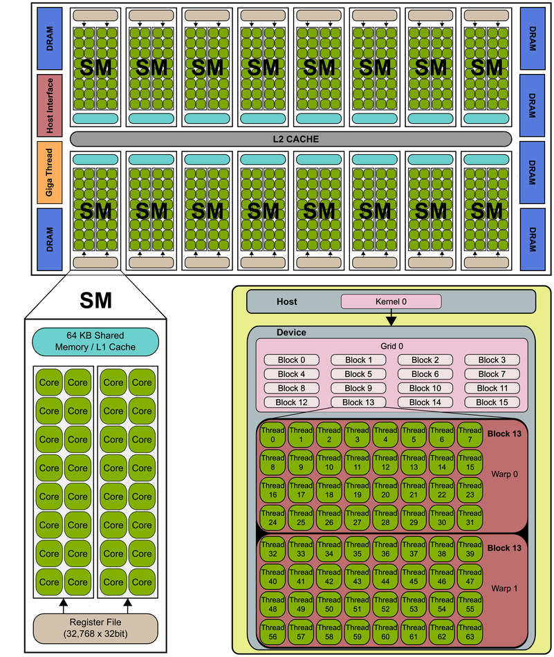 NVIDIA Fermi micro-architecture (src)
CUDA
Scientists/tinkerers started using GPUs for non-graphics problems that fit the SIMT paradigm, such as linear algebra (eventually ML/deep learning). A major issue with this was that they had to shoehorn their solutions to the graphics-oriented APIs exposed by GPUs.
In ~2006, NVIDIA comes up with CUDA, opening the doors to general purpose computing on GPUs.
CUDA mainly provides the ability to program the GPU using a set of extensions to C/C++, which are compiled
down to PTX (NVIDIA GPU’s instruction set)
using their proprietary compiler (nvcc).
It exposes the GPU hardware to the programmer as a grid of threads. Each grid is further divided into independently scheduled blocks of threads, each of which executes on a single SM.
The number of thread blocks executing a kernel function (a C/C++ function that executes on the GPU)
can be configured using the <<<NoOfBlocks, NoOfThreads>>> syntax.
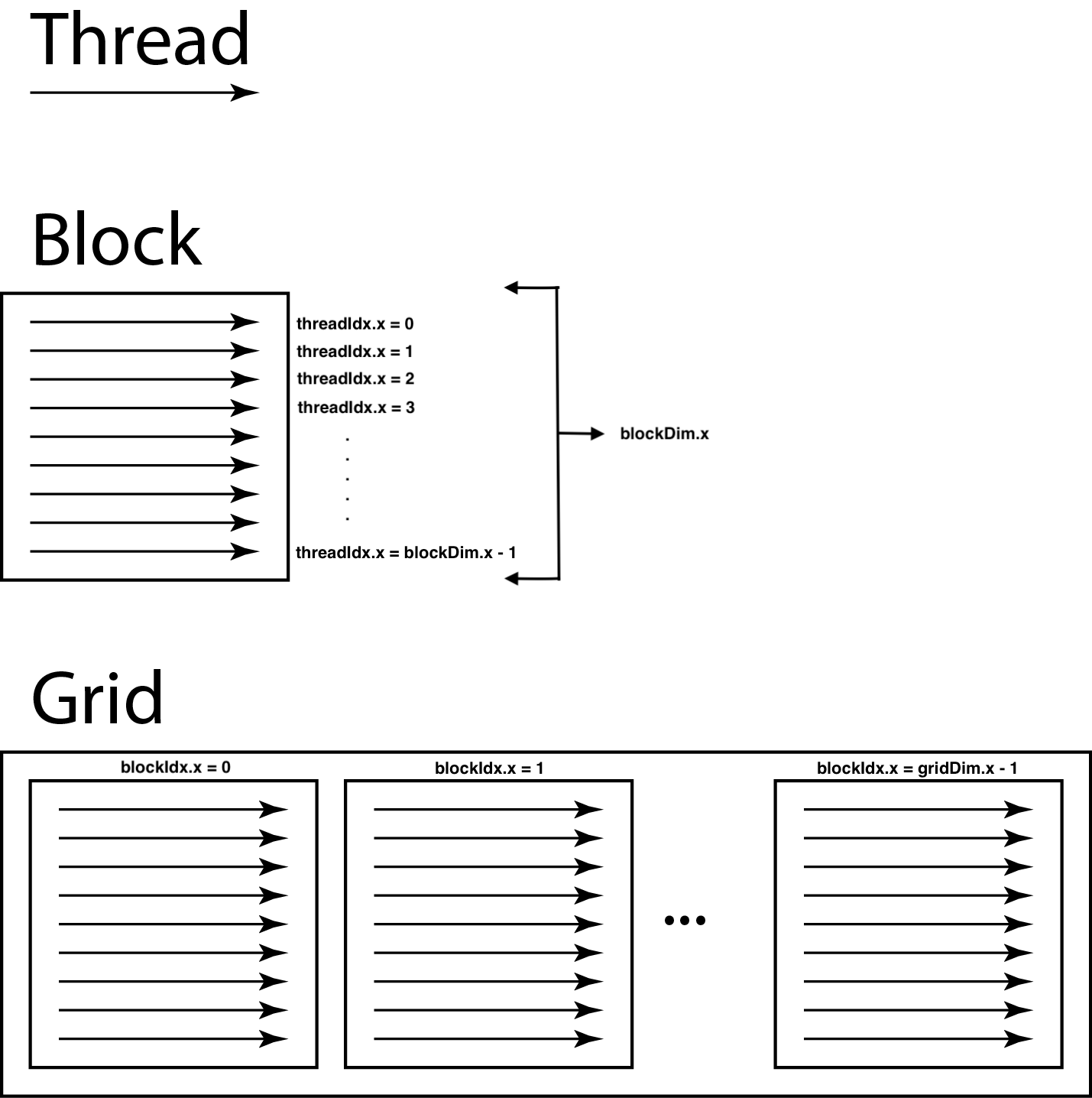 GPU grids (original src)
Note: CUDA is only available on NVIDIA graphics cards. OpenCL is the vendor independent equivalent, although CUDA has a larger amount of support/documentation/libraries.
simple example
// compile using `nvcc example.cu`
#include <cuda.h>
#include <stdio.h>

__global__ void vecAddKernel(float *A, float *B, float *C, int n) {
  int i = blockDim.x * blockIdx.x + threadIdx.x;
  if (i < n)
    C[i] = A[i] + B[i];
}

void vecAdd(float *h_A, float *h_B, float *h_C, int n) {
  int size = n * sizeof(float);
  float *d_A, *d_B, *d_C;

  cudaMalloc((void **)&d_A, size);
  cudaMemcpy(d_A, h_A, size, cudaMemcpyHostToDevice);
  cudaMalloc((void **)&d_B, size);
  cudaMemcpy(d_B, h_B, size, cudaMemcpyHostToDevice);
  cudaMalloc((void **)&d_C, size);

  vecAddKernel<<<ceil(n / 256.0), 256>>>(d_A, d_B, d_C, n);

  cudaMemcpy(h_C, d_C, size, cudaMemcpyDeviceToHost);

  cudaFree(d_A);
  cudaFree(d_B);
  cudaFree(d_C);
}

int main() {
  float a[] = {1, 2, 3, 4};
  float b[] = {1, 2, 3, 4};
  float c[] = {0, 0, 0, 0};

  vecAdd(a, b, c, 4);
  for (int i = 0; i < 4; i++) {
    printf("%f ", c[i]);
  }
  printf("\n");
}
example from Programming Massively Parallel Processors
vecAdd above is a normal C/C++ function that:
- allocates memory on the GPU (
cudaMalloc) - copies the required data from the CPU DRAM (called host memory in CUDA terminology) to the GPU DRAM (device memory) using
cudaMemcpy - calls the kernel function with a set number of thread blocks of equal size
- copies the computed results back to the CPU DRAM (
cudaMemcpy) - frees GPU DRAM (
cudaFree)
vecAddKernel is a kernel function (indicated by __global__) that adds vectors A, B and
stores them in C.
This kernel gets executed by ceil(n / 256.0) blocks, each consisting of 256 threads.
Since each thread is called with the same arguments, it uses some of the CUDA built-in variables
(that provide the position of the thread in its grid) to choose the index that it should operate on.
Finally, the if condition prevents out of bounds access in case the data size is not evenly
divisible by the threads in each block (blockDim).
VGG16
VGGNet is a simple CNN (Computational Neural Network) architecture, put forward by the Visual Geometry Group at Oxford in 2014. The version with 16 weight layers (13 convolution + 3 fully connected layers), called VGG16 is available pretrained (on ImageNet) from Tensorflow.
I first wrote a simple python version of the VGG16 inference to make sure that my output matches with that of tensorflow.
import numpy as np
import tensorflow as tf
from PIL import Image

# from https://github.com/keras-team/keras/blob/07e13740fd181fc3ddec7d9a594d8a08666645f6/keras/applications/imagenet_utils.py#L168-L238
def preprocess_img(img):
    x = img.astype(np.float32)
    # 'RGB'->'BGR' (because of opencv?)
    x = x[..., ::-1]
    mean = [103.939, 116.779, 123.68]
    x[..., 0] -= mean[0]
    x[..., 1] -= mean[1]
    x[..., 2] -= mean[2]
    return x

# read sample image using PIL and resize to the size required by VGG16
img = np.asarray(Image.open('images/n02504458_12101.jpeg').resize((224, 224)))

# preprocess input image as done by tensorflow
img = preprocess_img(img)

# create tensorflow model
model = tf.keras.applications.vgg16.VGG16()

# get class probabilities
tfoutput = model.predict(img[np.newaxis, ...])[0]
To get the class labels corresponding to the highest probability outputs from the model, I saved
the class number to label mapping for ImageNet into a dictionary called IMAGENET_LABELS in labels.py and
imported it.
# from https://gist.github.com/yrevar/942d3a0ac09ec9e5eb3a#file-imagenet1000_clsidx_to_labels-txt
from labels import IMAGENET_LABELS

# return top predictions with probabilities from output of last layer
def get_top_predictions(preds, top=5):
    return {IMAGENET_LABELS[x]: preds[x] for x in (-preds).argsort()[:top]}
>>> get_top_predictions(tfoutput)
{'fur coat': 0.98191327,
 'Labrador retriever': 0.006128772,
 'Eskimo dog, husky': 0.0019237188,
 'golden retriever': 0.0015210236,
 'pug, pug-dog': 0.0012324217}
python implementation
The first step for the numpy implementation is to get the pretrained weights. The tensorflow model weights are available as a hdf5 file, which is a dictionary-like object with the layer names as the key and the weights and biases as the value for that layer.
import h5py
# from https://storage.googleapis.com/tensorflow/keras-applications/vgg16/vgg16_weights_tf_dim_ordering_tf_kernels.h5
VGG_WTS = h5py.File("vgg16_weights_tf_dim_ordering_tf_kernels.h5", "r")

# layer names from https://github.com/keras-team/keras/blob/v2.9.0/keras/applications/vgg16.py#L43-L227
# can also be obtained by executing `model.summary()` on the `Model` object
VGG_LAYERS = ['block1_conv1', 'block1_conv2', 'block1_pool',
              'block2_conv1', 'block2_conv2', 'block2_pool',
              'block3_conv1', 'block3_conv2', 'block3_conv3', 'block3_pool',
              'block4_conv1', 'block4_conv2', 'block4_conv3', 'block4_pool',
              'block5_conv1', 'block5_conv2', 'block5_conv3', 'block5_pool',
              'flatten',
              'fc1', 'fc2',
              'predictions']
Next, we write the activation functions: ReLU for the hidden layers and softmax for the output layer:
def relu(x):
    return np.maximum(x, 0)

def softmax(x):
    exp = np.exp(x)
    return exp / np.sum(exp)
Now, we can proceed to implement the 2D convolution operation. The inputs required for this will be the layer weights, biases and the output from the previous layer. Before proceeding, lets check the shapes of these inputs for the first layer.
# for the first layer, input is the image
>>> img.shape
(224, 224, 3)

# weights and biases for first CONV layer
>>> w, b = VGG_WTS[VGG_LAYERS[0]].values()

# the first layer of VGG16 is:
# x = layers.Conv2D(64, (3, 3), activation='relu', padding='same', name='block1_conv1')
# 64 kernels of size 3x3 with padding to make sure output has same size as input

# 64 3x3 kernels (1 per input channel: corresponds to the 3rd 3 below)
>>> w.shape
(3, 3, 3, 64)

# 1 bias per kernel
>>> b.shape
(64,)
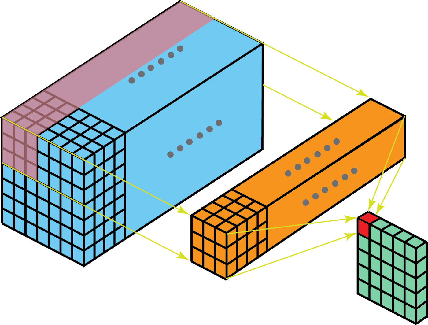 Convolution with 1 kernel (src)
In the above image, the blue cuboid corresponds to an output from one of the layers (feature map), which is being convolved with a single kernel (orange cuboid) to form 1 channel of the output.
The implementation follows:
def applyConv2d(w, b, inp):
    """assuming odd-sized square kernel"""
    ksize = w.shape[0]
    out_channels = w.shape[-1]

    # pad the input, not output: https://stackoverflow.com/a/69544897
    padded_inp = np.pad(inp, ((ksize//2, ksize//2),
                              (ksize//2, ksize//2),
                              (0, 0)))

    # output is same shape as input with more channels
    out = np.zeros(inp.shape[:2] + (out_channels,), dtype=np.float32)

    # convolve the surrounding of each pixel (3x3x3) with the kernel
    for x in range(inp.shape[0]):
        for y in range(inp.shape[1]):
            for c in range(out_channels):
                out[x][y][c] = np.tensordot(w[..., c],
                                            padded_inp[x:x+ksize, y:y+ksize],
                                            ksize)

    # add bias to each output channel
    for c in range(out_channels):
        out[..., c] += b[c]

    # apply relu activation
    return relu(out)
Each convolutional block of VGG16 ends with a max pooling layer, which is used to reduce the dimensions of the intermediate feature maps. The VGG16 max pooling is quite simple to implement since it uses a 2x2 kernel with a stride of 2, which reduces both the height and width of the feature map to half its original value. For instance, in the first block, max pooling reduces the feature map from (224, 224, 64) to (112, 112, 64).
def applyMaxPool2d(inp):
    """2x2 kernel with (2,2) stride"""
    out = np.zeros((inp.shape[0]//2, inp.shape[1]//2, inp.shape[2]), dtype=np.float32)
    for x in range(out.shape[0]):
        for y in range(out.shape[1]):
            for c in range(inp.shape[2]):
                out[x][y][c] = np.max(inp[2*x:2*(x+1), 2*y:2*(y+1), c])
    return out
Lastly, we write a function to apply all layers of VGG16 to the input image:
def applyVgg16(inp):
    curr = inp
    outputs = []
    for layer in VGG_LAYERS:
        if "pool" in layer:
            out = applyMaxPool2d(curr)
        elif layer == "flatten":
            out = curr.flatten()
        # weight layers
        else:
            w, b = (np.array(x) for x in VGG_WTS[layer].values())
            if layer.startswith("fc") or layer == "predictions":
                # fully connected layers are a simple matrix multiplication
                out = np.matmul(w.T, curr.reshape(-1, 1)).flatten() + b
                out = relu(out) if layer.startswith("fc") else softmax(out)
            else:
                out = applyConv2d(w, b, curr)
        outputs.append(out)
        print(f"processed {layer}: inshape: {curr.shape}, outshape: {out.shape}")
        curr = out

    # return output of all hidden layers along with output layer
    # helps in inspecting output of hidden layers
    return outputs
Now we call the above function on the preprocessed image and print the predictions:
start = datetime.datetime.now()
outputs = applyVgg16(img)
end = datetime.datetime.now()

print("predictions: ", get_top_predictions(outputs[-1]))
print(f"in {end-start}")
$ ./numpy_vgg16.py
processed block1_conv1: inshape: (224, 224, 3), outshape: (224, 224, 64)
processed block1_conv2: inshape: (224, 224, 64), outshape: (224, 224, 64)
processed block1_pool: inshape: (224, 224, 64), outshape: (112, 112, 64)
processed block2_conv1: inshape: (112, 112, 64), outshape: (112, 112, 128)
processed block2_conv2: inshape: (112, 112, 128), outshape: (112, 112, 128)
processed block2_pool: inshape: (112, 112, 128), outshape: (56, 56, 128)
processed block3_conv1: inshape: (56, 56, 128), outshape: (56, 56, 256)
processed block3_conv2: inshape: (56, 56, 256), outshape: (56, 56, 256)
processed block3_conv3: inshape: (56, 56, 256), outshape: (56, 56, 256)
processed block3_pool: inshape: (56, 56, 256), outshape: (28, 28, 256)
processed block4_conv1: inshape: (28, 28, 256), outshape: (28, 28, 512)
processed block4_conv2: inshape: (28, 28, 512), outshape: (28, 28, 512)
processed block4_conv3: inshape: (28, 28, 512), outshape: (28, 28, 512)
processed block4_pool: inshape: (28, 28, 512), outshape: (14, 14, 512)
processed block5_conv1: inshape: (14, 14, 512), outshape: (14, 14, 512)
processed block5_conv2: inshape: (14, 14, 512), outshape: (14, 14, 512)
processed block5_conv3: inshape: (14, 14, 512), outshape: (14, 14, 512)
processed block5_pool: inshape: (14, 14, 512), outshape: (7, 7, 512)
processed flatten: inshape: (7, 7, 512), outshape: (25088,)
processed fc1: inshape: (25088,), outshape: (4096,)
processed fc2: inshape: (4096,), outshape: (4096,)
processed predictions: inshape: (4096,), outshape: (1000,)
predictions:  {'African elephant, Loxodonta africana': 0.9346673, 'tusker': 0.06419284, 'Indian elephant, Elephas maximus': 0.0011378175, 'warthog': 6.19383e-07, 'water buffalo, water ox, Asiatic buffalo, Bubalus bubalis': 3.1221526e-07}
computed in 0:02:46.589266
So, our pure numpy VGG16 inference implementation takes around 3 minutes to process 1 image.
Now lets see how much this could be sped up with a naive CUDA implementation of the slow operations (convolution).
speed up using CUDA
The first task to use CUDA is to divide the problem into (gridDimension, blockDimension) sized sub-problems.
Since the number of threads in a block is limited to 1024 and the number of output channels of any layer in
VGG16 does not exceed 512, we can set the blockDim to the output channel count for each layer.
The gridDim can be set to the image/feature map (height, width).
import pycuda.gpuarray
import pycuda.driver as cuda
import pycuda.autoinit

def applyConv2dCuda(w, b, inp):
    ksize = w.shape[0]
    inp_channels = inp.shape[-1]
    out_channels = w.shape[-1]
    padded_inp = np.pad(inp, ((ksize//2, ksize//2),
                              (ksize//2, ksize//2),
                              (0, 0)))
    out = np.zeros(inp.shape[:2] + (out_channels,), dtype=np.float32)

    # convert numpy arrays to pycuda.gpuarray
    in_gpu, out_gpu = pycuda.gpuarray.to_gpu(padded_inp), pycuda.gpuarray.to_gpu(out)
    w_gpu, b_gpu = pycuda.gpuarray.to_gpu(w), pycuda.gpuarray.to_gpu(b)

    # call cuda implementation with the GPU arrays
    cudaConv2d(in_gpu, out_gpu, w_gpu, b_gpu, np.int32(inp_channels), np.int32(ksize),
               block=(out_channels, 1, 1), grid=inp.shape[:2])

    # copy back the output from GPU memory
    return out_gpu.get()
The setup code to call the cuda function cudaConv2d is similar to the example we looked at earlier.
In this case, pycuda provides us an easy way to copy numpy ndarray-like data from the CPU to the GPU using its
GPUArray class.
Now, we write our CUDA code for convolution. The below kernel calculates the value of 1 pixel in the output feature map of a layer.
The most convoluted part here is the calculation of the indices into the various input arrays, since all of them are multi-dimensional, but represented by a single-dimensional array in C++.
I encountered an error cuMemFree failed: an illegal memory access was encountered, which was likely due
to out of bounds access into the input array. Fortunately, NVIDIA kernels support printf, which made debugging
these issues easier.
__global__ void conv2d(const float *inp, float *out, const float *w,
                       const float *b, int inp_channels, int ksize) {
  int channel_num = threadIdx.x;
  int out_channels = blockDim.x;

  // pixel (x, y)
  int x = blockIdx.x;
  int y = blockIdx.y;

  int outidx = out_channels * gridDim.y * x +
               out_channels * y +
               channel_num;

  for (int i = 0; i < ksize; i++) {
    for (int j = 0; j < ksize; j++) {
      for (int k = 0; k < inp_channels; k++) {

        // w is 4D with dimensions: (ksize, ksize, input_channels, output_channels)
        int widx = (ksize * inp_channels * out_channels * i) +
                   (inp_channels * out_channels * j) +
                   (out_channels * k) +
                   channel_num;

        // inp is 3D with dimensions: (blockDim.x + padding, blockDim.y + padding, input_channels)
        int inpidx = ((gridDim.y + ksize - 1) * inp_channels * (i + x)) +
                     (inp_channels * (j + y)) +
                     k;

        out[outidx] += inp[inpidx] * w[widx];
      }
    }
  }

  // add bias
  out[outidx] += b[channel_num];

  // relu
  if (out[outidx] < 0) {
    out[outidx] = 0.0;
  }
}
To be able to compile and run this CUDA code at runtime, we provide the above code as a python string to
pycuda’s SourceModule
class
from pycuda.compiler import SourceModule

src = """...placeholder for CUDA code..."""
mod = SourceModule(src)
cudaConv2d = mod.get_function("conv2d")
Finally, after executing this, we obtain the following output which is the same as the one from tensorflow and our numpy implementation. The pycuda implementation however completes in ~5 seconds which is ~30x faster than our CPU based numpy implementation.
Tensorflow on the other hand is even faster than our implementation at ~1 second. This would most likely be because it internally uses the cuDNN library, which is highly optimized for deep neural network operations.
$ ./pycuda_vgg16.py
processed block1_conv1: inshape: (224, 224, 3), outshape: (224, 224, 64)
processed block1_conv2: inshape: (224, 224, 64), outshape: (224, 224, 64)
processed block1_pool: inshape: (224, 224, 64), outshape: (112, 112, 64)
processed block2_conv1: inshape: (112, 112, 64), outshape: (112, 112, 128)
processed block2_conv2: inshape: (112, 112, 128), outshape: (112, 112, 128)
processed block2_pool: inshape: (112, 112, 128), outshape: (56, 56, 128)
processed block3_conv1: inshape: (56, 56, 128), outshape: (56, 56, 256)
processed block3_conv2: inshape: (56, 56, 256), outshape: (56, 56, 256)
processed block3_conv3: inshape: (56, 56, 256), outshape: (56, 56, 256)
processed block3_pool: inshape: (56, 56, 256), outshape: (28, 28, 256)
processed block4_conv1: inshape: (28, 28, 256), outshape: (28, 28, 512)
processed block4_conv2: inshape: (28, 28, 512), outshape: (28, 28, 512)
processed block4_conv3: inshape: (28, 28, 512), outshape: (28, 28, 512)
processed block4_pool: inshape: (28, 28, 512), outshape: (14, 14, 512)
processed block5_conv1: inshape: (14, 14, 512), outshape: (14, 14, 512)
processed block5_conv2: inshape: (14, 14, 512), outshape: (14, 14, 512)
processed block5_conv3: inshape: (14, 14, 512), outshape: (14, 14, 512)
processed block5_pool: inshape: (14, 14, 512), outshape: (7, 7, 512)
processed flatten: inshape: (7, 7, 512), outshape: (25088,)
processed fc1: inshape: (25088,), outshape: (4096,)
processed fc2: inshape: (4096,), outshape: (4096,)
processed predictions: inshape: (4096,), outshape: (1000,)
predictions:  {'African elephant, Loxodonta africana': 0.9346673, 'tusker': 0.06419284, 'Indian elephant, Elephas maximus': 0.0011378153, 'warthog': 6.193812e-07, 'water buffalo, water ox, Asiatic buffalo, Bubalus bubalis': 3.1221467e-07}
computed in 0:00:04.784639
To optimize further, we could also write the max pooling algorithm using CUDA, but the speed up won’t be as pronounced as the conv2d case.
Hopefully this simple implementation helps to demystify how deep learning/ML libraries get such incredible speedups when using GPUs (or TPUs on Google Colab)!
Note: execution was done on a Intel i9-9900X processor with a NVIDIA RTX 2060 GPU. code is available on github.